
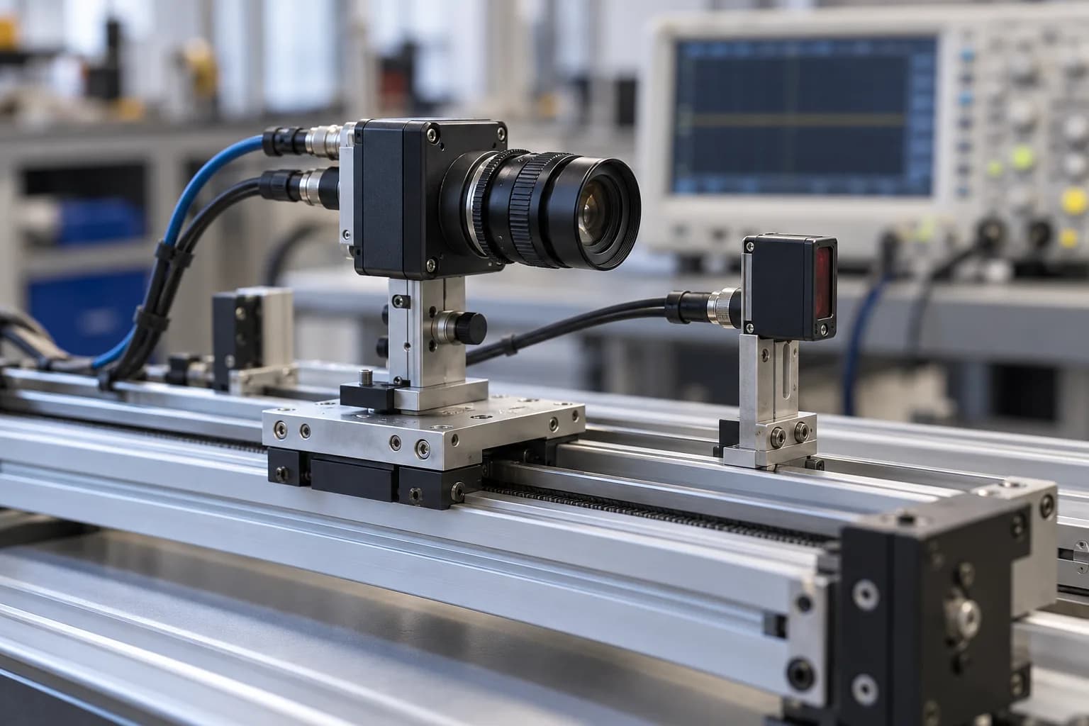
Two correct readings may describe different events
A camera may correctly observe an object and a distance sensor may accurately measure its own sample. If those observations describe different moments, their combination can still be wrong. The defect lies in the association rule rather than either sensor's precision. Slow laboratory motion may conceal it until the actual operating speed is used. Integration therefore extends beyond connectors and message formats to timing, position, calibration and decision context.
A record arriving now may represent an old event. Network queues, buffer replay and retries can make stale observations appear current. Combining images with physical measurements requires separate event and arrival times. The decision process also needs defined behavior for missing observations or uncertain clocks. Filling gaps with an undocumented assumption prevents the accuracy of individual sensors from carrying through to the integrated system.
Which instant does the timestamp represent?
A timestamp may denote exposure start, exposure midpoint, data-ready interrupt, driver read or packet transmission. These are not equivalent. The physical acquisition interval must be distinguished from the moment software sees the record. Effects such as row-wise camera readout can add motion-dependent differences. Documentation, driver inspection and experiments establish timestamp meaning; a field named timestamp does not independently tell a downstream application which instant it represents.
The interface contract states units, clock source and epoch. Wall time cannot be directly compared with a counter since device boot. Wraparound and reboot identity also matter. A monotonic clock helps measure durations, but independent monotonic counters do not share a reference. Records retain the conversion to a common time base and its uncertainty, preventing later consumers from inventing assumptions that were never justified at acquisition.
Clock offset and clock drift require different treatment
A fixed difference may be corrected with an offset, but clocks running at different rates make that correction age. A hypothetical relative rate error of 20 ppm accumulates 36 ms in 30 minutes. That is an illustrative calculation, not a device specification. Engineering defines resynchronization frequency and how time uncertainty grows during disconnection. A successful initial alignment cannot establish that two streams remain aligned for an entire operating day.
Network clock synchronization, physical triggering and a shared hardware clock are different options. None establishes a precision level merely by being named. Asymmetric network delay can affect offset estimates, and backward wall-clock corrections can disrupt ordering. Sequence counters help preserve event order. The choice depends on timing requirements and hardware access. NTP availability alone cannot prove that a pair of sensors acquired their physical observations at matching instants.
Section references: RFC 5905 · Network Time Protocol ↗
How does a 25 ms timing error become a 50 mm position error?
For constant linear speed, displacement is approximately Δx = v × Δt. At a hypothetical 2 m/s, a 25 ms association error corresponds to 50 mm. Even a much more precise sensor can then be matched to the wrong surface or object. A 3 ms timing uncertainty corresponds to 6 mm at that speed. The simple model excludes rotation, acceleration and viewing geometry, which require an expanded budget when relevant.
Delay and uncertainty are different. A fixed, known 100 ms transport delay may be manageable in offline analysis, while a few unknown variable milliseconds can limit physical association. For real-time decisions, even known latency matters because the action becomes stale. Accuracy and response-time budgets therefore remain distinct but are evaluated together. Acquisition time and action time answer different questions; one average latency cannot explain both properties.
| Timing difference | Displacement | Meaning |
|---|---|---|
| 3 ms | 6 mm | Even small timing uncertainty can matter |
| 25 ms | 50 mm | Risk of associating different events |
| 36 ms | 72 mm | 20 ppm over 30 minutes example |
Nearest-time matching needs an explicit policy
Approximate-time tools help associate message streams, but engineering requirements determine a suitable tolerance. A wide window accepts mismatched events; a narrow one drops valid pairs. Queue size, out-of-order arrival and late-data behavior require explicit choices. ROS message_filters provides an implementation reference. Using a synchronizer does not establish that clocks share a reference or that its selected tolerance is physically adequate for the motion and decision involved.
The example below searches source timestamps for one query, subtracts a known offset, rejects out-of-window candidates and declines an exact tie. Arrival time is not used for association. It is neither a complete multi-stream buffer nor a clock estimator; offset is assumed to have been measured elsewhere. Real systems also need sample-consumption rules, queue cleanup and ownership across multiple matches. Those concerns remain outside this intentionally bounded example.
const assert = require('node:assert/strict');
// One query against source timestamps; not a multi-stream queue implementation.
function pairAt(eventMs, samples, clockOffsetMs, toleranceMs) {
  assert([eventMs, clockOffsetMs, toleranceMs].every(Number.isFinite));
  assert(toleranceMs >= 0);
  assert(samples.every(s => Number.isFinite(s.sourceMs)));
  const ranked = samples.map(sample => ({
    sample,
    deltaMs: Math.abs(sample.sourceMs - clockOffsetMs - eventMs),
  })).sort((a, b) => a.deltaMs - b.deltaMs);
  if (!ranked.length || ranked[0].deltaMs > toleranceMs) return null;
  if (ranked[1] && ranked[0].deltaMs === ranked[1].deltaMs) return null;
  return ranked[0];
}
const samples = [
  { id: 'sync-probe-a', sourceMs: 1025, arrivalMs: 5000 },
  { id: 'sync-probe-b', sourceMs: 1045, arrivalMs: 1060 },
];
assert.equal(pairAt(1000, samples, 25, 10).sample.id, 'sync-probe-a');
assert.equal(pairAt(1000, samples, 0, 10), null);
assert.equal(pairAt(5000, samples, 25, 10), null);
assert.equal(pairAt(1000, [
  { sourceMs: 995 }, { sourceMs: 1005 },
], 0, 10), null); // Ambiguous nearest match is not silently selected.
assert.equal(pairAt(1000, [], 0, 10), null);
assert.throws(() => pairAt(1000, samples, 0, -1));
const spatialErrorMm = speedMps => delayMs => speedMps * delayMs;
assert.equal(spatialErrorMm(2)(25), 50);
const driftMs = 20e-6 * 30 * 60 * 1000;
assert(Math.abs(driftMs - 36) < 1e-10);
assert(Math.abs(spatialErrorMm(2)(driftMs) - 72) < 1e-10);
console.log('Offset, ambiguity, stale query and drift examples pass');
Section references: ROS 2 message_filters · Approximate Time Synchronizer ↗
Sampling and calibration do not eliminate timing error
A nominal 100 Hz rate does not guarantee exact 10 ms spacing or instantaneous acquisition. Triggering, integration duration and driver buffering need review. Nearest-sample selection adds mismatch; linear interpolation assumes sufficiently smooth evolution. At a sharp transition, interpolation can create a value that never physically occurred. Each method must be evaluated against signal bandwidth, motion and the actual sampling arrangement rather than chosen solely because it produces a complete table.
Spatial calibration remains a separate variable. Perfectly timed sensors can still combine incorrectly if axes or mounting transforms are wrong. Records retain calibration versions, and remounted hardware must not silently reuse stale parameters. Static targets can investigate geometry while controlled motion helps expose timing errors. Both experiments state conditions and reference uncertainty. One end-to-end score often cannot identify which underlying error source requires correction.
Which faults should the bench deliberately inject?
Bench scenarios include fixed offset, increasing drift, missing samples, duplicates, out-of-order arrival and restart. Each has an expected match or rejection behavior. Delaying packets and changing physical acquisition time are different tests and should be injected separately. Controlled motion needs known speed and timing references. The plan also defines whether rejected ambiguous pairs count as data loss, appropriate abstention or a separate quality condition.
Review difficult slices and rejected records alongside average matching error. An average over accepted pairs can improve artificially if difficult cases are simply discarded. Report coverage, latency and error together. Long runs expose clock drift while load tests reveal queues. Laboratory evidence remains bounded by hardware, temperature and driver version; it cannot establish identical behavior in every field environment or after an undocumented software update.
- Are timestamp meaning, units and clock source documented?
- Were offset, drift and sampling effects tested separately?
- Is arrival time kept separate from event time?
- Are ambiguous and missing pairs rejected visibly?
Trace a decision back to raw observations
A decision record retains identifiers for both observations, source times, time conversion and calibration version. Investigators can inspect the association rather than only the final number. Raw-data retention and sharing follow the project scope. Quality flags must survive central processing; presenting every observation with equal confidence removes uncertainty from the report without correcting the physical error. Review requires access to the relevant acquisition context.
Recorded observations can be reprocessed with a revised association method while preserving earlier result versions. This gives hardware and software teams a shared basis for investigation. A driver fix that changes timestamp semantics can also change a model or alarm. Integration acceptance is therefore repeated after relevant sensor, firmware, mounting or processing changes, rather than being treated as a one-time check at initial installation.
Gokbilge Tech's contribution to sensor integration
Gokbilge Tech connects electrical interfaces, firmware, timing and application data in sensor integration. Local board and systems knowledge supports the use of sourced sensors in defined tasks. Optoelectronic and simulation-hardware work provide relevant capabilities for controlled experiments. These links do not establish compatibility with every sensor brand or promise a particular synchronization precision. Performance depends on assessment of the selected arrangement and its operating conditions.
An initial discussion can use sample data, motion speed, decision deadlines and the current clock arrangement. The next steps define an error budget, interface contract and bench experiment, separating timing problems from perception or modeling problems where needed. The examples do not disclose a private customer project. The service is scoped as measurable systems engineering that explains and addresses why individually plausible components can behave incorrectly when combined.
Technical references
Want to apply this approach to your system?
Discuss your technical requirements →